Ben North, September 2016
This write-up assumes some level of background knowledge of the Lorenz cipher machine and the attacks automated by Colossus. The Wikipedia article gives a good description, as does the source material provided by the General Report on Tunny (henceforth GRT).
The motivation for this study came in two parts:
The book Colossus: The secrets of Bletchley Park's code-breaking computers has an appendix written by William T. Tutte, 'My Work at Bletchley Park'. Tutte was the Bletchley Park codebreaker who, in what has been called 'one of the greatest intellectual feats of World War II', reverse-engineered the structure of the Lorenz cipher machine just from a sample of key. In this appendix, he writes (p.368, emphasis added):
Having got a key K, we can write
But Δ(ψ1 + ψ2) is about 70 per cent dot. ['Dot' is the term used for a binary zero.] Hence Δ(K1 + K2) must be in 70 per cent agreement with Δ(χ1 + χ2). And the agreement would still be 70 percent for other pairs of impulses. Surely with 1000 or so letters of key the rectangle method would have resolved Δ(K1 + K2) into Δχ1 and Δχ2? I suppose I could check this if I went to enough trouble. But what would be the point now, so long after the last Fish message was sent? On second thoughts the problem could be reformulated as one in pure mathematics and so made worth solving. It would not be the first of Bletchley's little problems to undergo such a transformation.Δ(K1 + K2) = Δ(χ1 + χ2) + Δ(ψ1 + ψ2).
I thought the emphasised question was an interesting one.
GRT explains the procedures and formulae used in recovering the χ wheels from ciphertext, and they struck me as very similar to the Belief Propagation algorithm used for decoding LDPC codes. I thought it would be interesting to more properly compare the two methods, and also to ask whether Belief Propagation, first proposed in 1982, was an improvement over the methods used at Bletchley Park.
This study combines these points, and looks at chi-breaking from key under both the 'accurate convergence' described in GRT and the 'belief propagation' approach. Can we recover Δχ1 and Δχ2 from 1000 or so letters of K?
We can get a sanity-check sense for whether '1000 or so letters of key' will be sufficient to break χ1 and χ2 by looking at the information carried in one received bit of K12. We have to recover at most 72 bits (χ1 is of length 41; χ2 is of length 31; 'at most' because there are constraints on the patterns, described more fully below).
The received bit depends on the value of B, the 'dot'-biased noise term Δ(ψ1 + ψ2), as follows:
This is a 'binary symmetric channel', with capacity 1 − Hb(p), where Hb is the binary entropy function and p is the crossover probability, here 30%. In our case, then, the capacity is 1 − Hb(0·3) = 0·119. Receiving 1000 such values ought to provide 119 bits of information, then, which exceeds the 72 we require. So on the face of it, we do have enough information; but whether our decoding algorithm is good enough to extract it is another question.
The process of 'Rectangling' used at Bletchley Park for recovering the wheel patterns is described in detail in Chapter 24 of GRT, but to summarise:
The unknown χ1 wheel can be represented as a binary-valued vector of length 41 (indexed from 0 up to 40); similarly, the χ2 wheel by a 31-long vector. We can generate a 'χ stream', a time series of length-2 vectors whose first component is consecutive entries from χ1 and second χ2 by rotating these wheels (together) one bit-position at a time. We are interested in the streams Δχ1 and Δχ2, where Δχk(t) = χk(t) + χk(t − 1). (The 'delta' implies difference but in the xor-based arithmetic used, addition is the same as subtraction.) We are also interested in their sum, denoted Δχ12 = Δχ1 + Δχ2, which is cyclic of length 41 × 31 = 1271.
The model is that there is also a 'biased coin' B which produces 0 more often than it produces 1. We flip this coin independently for each t, and then observe a sequence of Δχ1(t) + Δχ2(t) + B(t).
The challenge is to recover Δχ1 and Δχ2. This is only possible up to the transformation which inverts all bits of both Δχ1 and Δχ2, because such a transformation would leave the observed Δχ12 unchanged. We do also have some constraints on the Δχ vectors; an immediate one is that such a vector must have an even number of 1s (otherwise it could not be 'integrated' to find χ), and see the discussion of 'legal wheels' below.
The 'biased coin' B can be:
If we are working with intercepted ciphertext, B is ΔD12, the sum of the first and second impulses of delta-de-χ (i.e., delta-ψ + delta-plain).
If, as pondered in the Tutte quote motivating this study, we are working with a section of key K recovered from a depth, B is Δψ12. Hence the equation in the quote:
Δ(K1 + K2) = Δ(χ1 + χ2) + Δ(ψ1 + ψ2).
In full, the information we have is a list of the observed Δχ1(t % 41) + Δχ2(t % 31) + B(t) values for 0 ≤ t < T, where T is the number of letters received.
Since all B(t) are independent, and because of the cyclic nature of the Δχ streams, we can reduce the information to just a difference of 'number of 0s − number of 1s' corresponding to each Δχ1(i) and Δχ2(j). If we receive fewer than 1271 letters, we'll receive no information for some (i, j) pairs.
The information we have is therefore a 'rectangle' of signed counts, called θ(i, j).
The following process for estimating the Δχ2 and Δχ1 vectors from the θ(i, j) rectangle is described in Section 24C of GRT, and was known as 'crude convergence'.
The idea was, approximately speaking: Hypothesise some vector of 41 values for Δχ1 (a 'start'). Then, for each j < 31, look at all the θ(i, j) for i < 41. Because B gives 0 more often than it gives 1, a positive θ(i, j) is evidence that Δχ12(i, j) = 0, i.e., that Δχ2(j) = Δχ1(i). A negative θ(i, j) is evidence that Δχ2(j) ≠ Δχ1(i).
Pretending for a minute that we know all Δχ1 values to be correct, then, this means:
Let ε1 be the vector which has the value +1 whenever Δχ1 = 0 and the value −1 whenever Δχ1 = 1. Then Σ i [ε1(i)θ(i, j)] is, in some sense, the total evidence that Δχ2(j) = 0. If this sum is negative, we should suspect that Δχ2(j) = 1.
In this way, we determine, on the preponderence of evidence, the most likely value of each Δχ2(j).
Then, fix that 31-long vector Δχ2 and run the same process in the other direction to estimate Δχ1. Repeat. The idea is that this process will converge to a good estimate of the two Δχ vectors.
The process of 'accurate convergence' handles the calculation in a more formal probabilistic setting, and derives a more accurate procedure. It tracks a continuous score for how likely each bit is to be zero or one, as opposed to just which value is more likely. The details are given in Section 24W(a) of GRT, but in summary:
First define ζ as the ratio P(B = 0) / P(B = 1), i.e., the factor by which it is more likely that B will yield 0 rather than 1. For our case, where 'Δ(ψ1 + ψ2) is about 70 per cent dot', we have ζ ≈ 2·33.
Then define the 'score' xi as the log-base-ζ-likelihood-ratio of the hypothesis 'Δχ1(i) = 0' (as compared to the alternative 'Δχ1(i) = 1'). Similarly, yj is the score of the hypothesis Δχ2(j) = 0. By alternating between
we obtain the following update rules:
\[y_j = \sum_i f(\theta_{ij}, x_i);\quad x_i = \sum_j f(\theta_{ij}, y_j)\] where \[f(k, l) = \log_\zeta \left(\frac{\zeta^{k+l} + 1}{\zeta^k + \zeta^l}\right).\]
The process of 'accurate convergence' performs these updates in turn until convergence of the signs of the scores, at which point the two Δχ vectors have been estimated.
It occurred to me that the rectangling problem is very similar to the decoding problem for Low-Density Parity Check error-correcting systems, in the following sense.
When rectangling, we have a large collection of bits for which:
and this is exactly the set-up for a LDPC code.
Expressing rectangling in LDPC terms, the transmitted bits are the individual Δχ1(i) and Δχ2(j), and also their (xor) sums Δχ12(i, j). We receive no direct information on any Δχ1(i) or Δχ2(j) but do have some noisy information on each Δχ12(i, j) — the θ(i, j) counts of excess zeros over ones. We can think of this as a situation where, in LDPC terms, we receive no data bits, and only have noisy information on the parity bits.
One popular decoding method for LDPC codes is Belief Propagation, one of a set of 'Factor Graph' algorithms. This paper gives a clear explanation of this class of algorithms:
In a Factor Graph setting, we view the LDPC decoding problem on a graph whose nodes are of three types: variables, checks, or observations. The graph's edges show which variables are related by parity checks, and which variable appears in which observation.
In our case, the parity checks arise from the definition of Δχ12:
Δχ12(i, j) = Δχ1(i) + Δχ2(j).
Equivalently,
Δχ1(i) + Δχ2(j) + Δχ12(i, j) = 0.
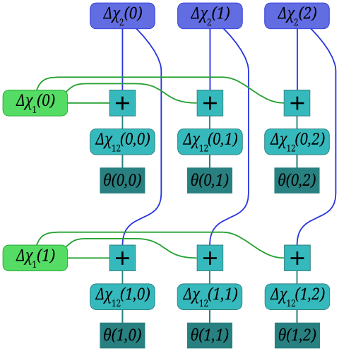
Our variables, then, are the 41 Δχ1 values, the 31 Δχ2 values, and the 1271 Δχ12 values. As a factor graph, we also have 'dongle' nodes for the observations θ(i, j) concerning Δχ12(i, j), and check nodes for the relationship between Δχ1(i), Δχ2(j), and Δχ12(i, j). For a simplified 2 × 3 case, the graph is:
Each square '+' node indicates that the variables connected to it must sum to zero.
The 'message passing' algorithm (see the KFL paper for details) gives update rules in terms of numerical messages passed between nodes. In our case, we use the log-base-\(\zeta\)-likelihood-ratio representation, and define xi to be the value of the Δχ1(i) node, which is the sum of that node's incoming messages. Similarly, yj is the value of the Δχ2(j) node. These scores mean exactly the same as the xi and yj scores of the Accurate Convergence scheme.
The computation performed by a variable node for the LLR representation is just to sum the incoming message values (p.512 of KFL).
The computation performed by each of our degree-three check nodes is via the function \[CHK(\lambda_1, \lambda_2) = \frac{1 + \lambda_1\lambda_2}{\lambda_1 + \lambda_2}.\] where \(\lambda\) are the likelihood ratio values (NB not the log-likelihood ratios). In terms of log-likelihood-ratio values k and l, then: \[CHK(k, l) = \log_\zeta\left(\frac{1 + \zeta^k\zeta^l}{\zeta^k + \zeta^l}\right).\] which is identical to the Bletchley Park \(f()\) function for accurate convergence; we will therefore rename it \(f\). This \(f\) function is only ever called with some θ(i, j) as one of its arguments; no messages get sent towards the 'dongle' node containing the observation θ(i, j).
We keep track of xi(j), the most recent message emitted by the variable node for Δχ1(i) along the edge to the check node that variable shares with Δχ2(j). The message value yj(i) is defined similarly. The messages into and out of a check node are:
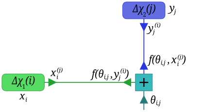
The score xi is the log-ζ-likelihood-ratio of 'Δχ1(i) = 0', and it is updated via the 31 incoming messages, to
\[x_i = \sum_{j=0}^{30} f(\theta_{ij}, y^{(i)}_j).\]
Note that this is almost the same as the Accurate Convergence update rule, except there the summand is f(θij, yj) rather than the f(θij, yj(i)) we have here.
The message yj(i), in turn, is the sum of all messages which Δχ2(j) receives over all other edges, i.e., all edges besides the one connecting it to Δχ12(i, j). Equivalently, yj(i) is the sum of all incoming messages (which is the score, yj) reduced by the message it received along the edge connecting it to Δχ12(i, j):
\[y^{(i)}_j = y_j - f(\theta_{ij}, x^{(j)}_i).\]
For a 'large' number of incoming edges, we might hope that the difference between yj and yj(i) would be small, in which case Belief Propagation and Accurate Convergence should behave very similarly.
The actual operational χ patterns were significantly constrained. The rules for a valid ('legal') χ pattern are described in Section 22B of GRT:
It seems that these extra constraints were important when χ-breaking; Section 25D(e) of GRT talks about adjusting candidate wheels to make them legal. Not many details are given, but we can imagine that an approach a little like the following might have been used. No doubt the methods used by the experienced codebreakers were more sophisticated.
Recall that we can only recover the delta-wheels up to the transformation which inverts all bits of both of them — that transformation preserves Δχ12, which is all we (noisily) observe. In view of this, we adopt the following steps for finding a pair of legal wheels 'close' to the converged estimate:
If the converged state (or its inverse) consists of two legal Δχ wheels, accept it.
Otherwise, use the magnitude of the xi scores (for Δχ1) and the yj scores (for Δχ2) to rank each wheel's bits in order from least certain to most certain, and take the least certain twelve for each wheel. Try flipping each single bit in turn; if that gives a legal Δχ wheel (or the inversion of one), add it to list of candidates for that wheel, noting the 'cost' (how much evidence was overruled), and whether the wheel needed to be inverted. Then try flipping two bits at a time, then three. Rank all candidates for each wheel from least costly to most.
Combine a candidate Δχ1 with a candidate Δχ2 such that either neither wheel is inverted or both are inverted. Accept the least costly candidate pair of wheels.
For the experiments described shortly, we need to be able to randomly generate legal wheels and evaluate the algorithms' performance on them. Section 25X of GRT notes that legal wheels may be enumerated by a process which, for the 41-long χ1 wheel, boils down to choosing ten integers, each between 1 and 4 inclusive, with sum 20; and another ten such with sum 21. These are the lengths of blocks of 0s and 1s.
The problem of randomly generating sets of ten such numbers, uniformly over all possibilities, turned out to be an interesting sub-project in the course of this study. I solved it by adapting the algorithm described in the paper Polynomial Time Perfect Sampler for Discretized Dirichlet Distribution (Matsui and Kijima) to incorporate an upper bound on the values each summand may take. I have not formally proved that the modified algorithm obeys all requirements to generate uniform samples, but I think it does, and the behaviour seems reasonable. For present purposes, then, it is certainly acceptable.
To explore these ideas, we can simulate the process of attemping to recover the two Δχ patterns as follows:
This simulation was performed 1,000,000 times, and the proportion of cases achieving at least N correct bits, for various N, was found. We are hoping for a high proportion of cases achieving a high number of correct bits.
The performance of the two algorithms, before and after legality enforcement, was as follows.
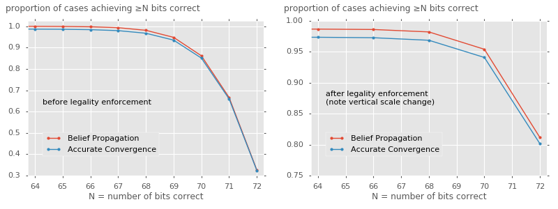
Left graph: Even before error correction using the legality constraint, both methods do well. They perfectly recover the wheel patterns around a third of the time, and 'almost' succeed (getting at most two bits wrong) a further half of the time. The Belief Propagation algorithm does very slightly better, although not meaningfully.
Right graph: After adjusting the recovered patterns so as to find a legal pair of wheel patterns, the 'perfect recovery' rate jumps to around 80% for each algorithm. The 'almost success' rate, allowing up to two wrong bits, jumps to around 95%. Note that we only ever get an even number of bits right, as an odd number of incorrect bits would mean one proposed delta-wheel would have an odd number of 1s, an impossibility.
These experiments have studied the most difficult pair of wheels, i.e., the longest ones. Breaking the shorter χ wheels would presumably be easier, with the algorithms achieving a higher success rate.
Although Belief Propagation does appear to perform slightly better than Accurate Convergence, I do not think it would have been useful to the codebreakers at Bletchley Park. The much greater amount of state required to run the algorithm (41 × 31 messages values rather than 41 + 31 scores) would make it impracticable to perform manually.
The detailed behaviour of the algorithms could be characterised more fully, but we have learnt enough to answer Tutte's question
Surely with 1000 or so letters of key the rectangle method would have resolved Δ(K1 + K2) into Δχ1 and Δχ2?
with 'very likely, yes'.
Available on github: bennorth/rectangling-ldpc.
Ben North, September 2016
This web-page content Copyright 2016 Ben North; licensed under CC BY-SA 4.0